
As discussed in our previous blog post on martingales and random walks, both concepts are fundamental in financial mathematics and quantitative finance. In financial modelling, however, the most relevant case is the random walk with drift. While it may seem at first that a random walk with drift has little in common with a martingale, the relationship between them is deeper than it appears. In this article, we explore the connection between random walks with drift, martingales, and the stochastic discount factor, to build a clearer understanding of what they truly are.
Table of Contents
- Martingales, Random Walks and Drifts
- From Drift to Martingale
- Link with the Stochastic Discount Factor
- Conclusion
- Further Reading
Martingales, Random Walks and Drifts
Let’s make some definitions here to ensure we all speak the same language (thank God mathematics is universal).

Martingale
A martingale $W_t$ with respect to a filtration $\mathcal{F}_t$ satisfies :
\[\mathbb{E}[W_{t+1} \mid \mathcal{F}_t] = w_t, \quad \forall t \ge 0.\]Intuitively, the best forecast of tomorrow’s value, given all information today, is simply today’s value.
Random Walk
A random walk $W_t$ is a discrete-time stochastic process defined by :
\[W_t = \sum_{i=1}^{t} \varepsilon_i,\]where ${\varepsilon_i}_{i \ge 1}$ is a sequence of i.i.d. random variables and where in many cases :
\[\mathbb{E}[\varepsilon_i] = 0, \quad \text{and} \quad \text{Var}(\varepsilon_i) = \sigma^2.\]In these settings, the process satisfies :
\[\mathbb{E}[W_{t+1} \mid \mathcal{F}_t] = W_t,\]which and the random walk $(W_t)$ is a martingale.
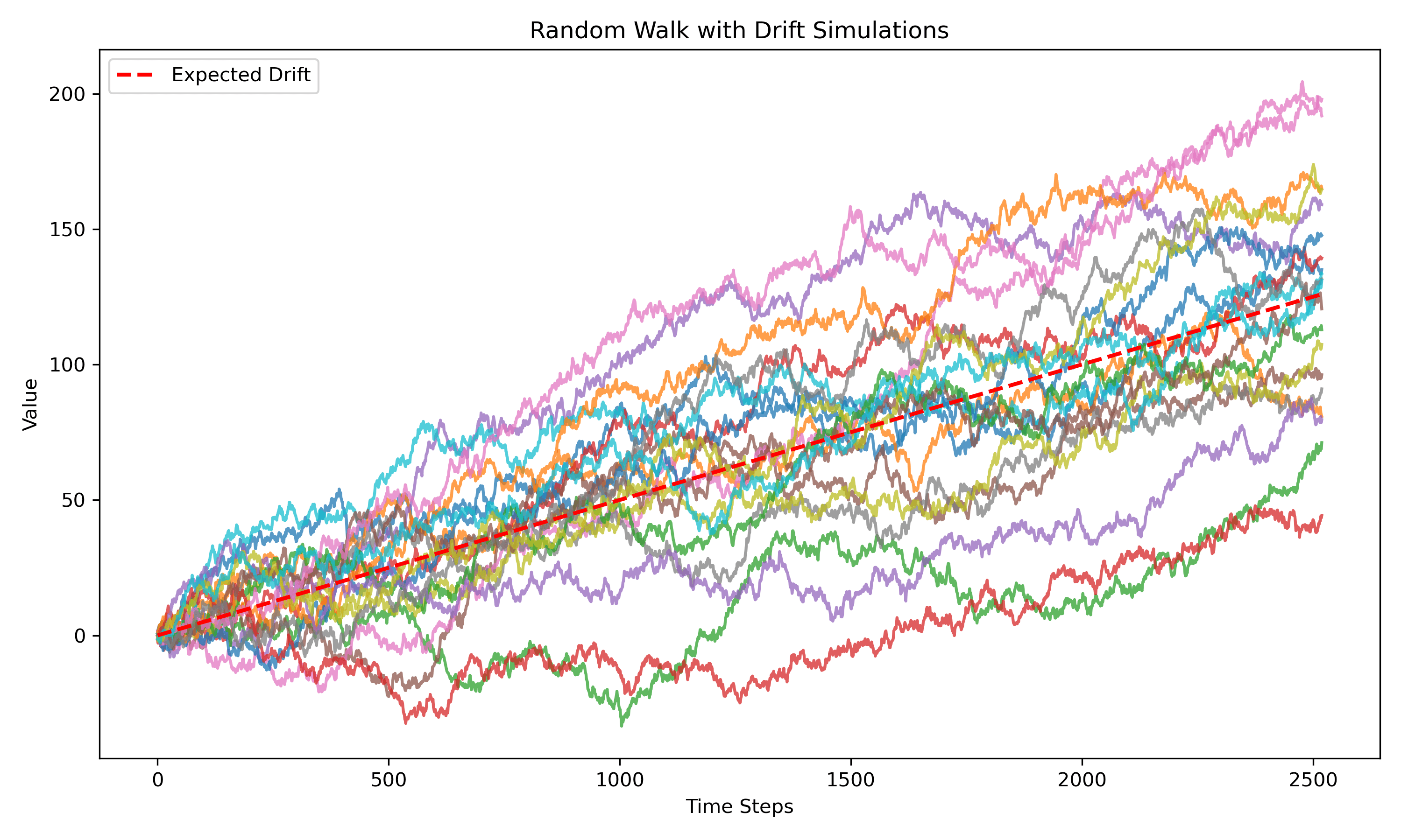
Random Walk with Drift
However, financial modelling requires more often than not to have $\mathbb{E}[\varepsilon_i] = r$, with $r$ a non null constant. To adjust, we can use $\tilde{\varepsilon_i} = \varepsilon_i - r$ to define a new random walk with increments $\tilde{\varepsilon_i}$ that we will note $\tilde{W_t}$. From the relationship we can say that $\tilde{W_t} = W_t - r \times t$ or equivalently $W_t = \tilde{W_t} + r \times t$.
Thus introducing a non zero constant for $\mathbb{E}[\varepsilon_i]$ creates a random walk with drift and modifies the process into : \(X_t = \mu t + W_t.\) This can be interpreted as a deterministic linear trend $\mu t$ plus a centered random walk $W_t$.
Quantitatively:
- The expected value evolves as $\mathbb{E}[X_t] = \mu t$ showing the systematic accumulation of the drift.
- The variance remains stochastic due to the random component : $\text{Var}(X_t) = t \sigma^2$
Hence, a random walk with drift is simply a martingale tilted by a linear deterministic trend $\mu t$.
In financial modeling, removing the drift by working under a risk-neutral measure recovers the martingale property crucial for pricing and arbitrage-free valuation.
import numpy as np
import matplotlib.pyplot as plt
np.random.seed(42)

N = 20          # number of sample paths
T = 2520        # number of time steps
mu = 0.05       # drift
sigma = 1       # volatility

eps = np.random.normal(mu, sigma, (T, N))
X = np.cumsum(eps, axis=0)  # random walk

expected_drift = np.arange(T) * mu

fig, ax = plt.subplots(figsize=(10, 6))
ax.plot(X, alpha=0.75,)
ax.plot(expected_drift, color='red', linestyle='--', linewidth=2, label='Expected Drift')

ax.set_title("Random Walk with Drift Simulations")
ax.set_xlabel("Time Steps")
ax.set_ylabel("Value")
ax.legend()

plt.tight_layout()
plt.show()
From Drift to Martingale
So far, we have described our random walks dynamics under a real-world measure, denoted by $\mathbb{P}$. Under $\mathbb{P}$, a random walk can exhibit a drift. When modelling financial instruments, this drift reflects required expected return for bearing risk. However it is far more convenient to work with martingales when computing expectations, the probability of a given event, … And that why mathematicals tools have been searched to transform random walk with drift into random walk : the change of measure, and more speciafically the risk-neutral measure in finance.
What is the key idea here ? Many real word applications require simply to compute an expectation. For a deriviative for instance, however the model used to describe the behavior of the underlying, Black Scholes for instance, we end up computed to expectation of the final payoff.
For any random real variable $X$, we can express it’s expectation as :
\[\mathbb{E}[X] = \int_{-\infty}^{\infty} f(x)x \mathrm{d}x\]Changing the measure simply means finding a new density function $f’$ for $X$ such that it becomes a martingale. How is this done rigorously ? That is where the Radon Nikodym Bridge comes by.
The Radon–Nikodym Bridge
The Radon–Nikodym Theorem is the key demonstration behind everything that will follow. Using the Radon Nikodyn variable
\(\Lambda_t = \frac{d\mathbb{Q}}{d\mathbb{P}}\Big|_{\mathcal{F}_t}.\)
sometimes called the change-of-measure density, reweights probabilities such that expectations under $\mathbb{P}$ are transformed into expectations under $\mathbb{Q}$:
Let’s give an intuition for what will happend if use it to transform our random walk with a positive drift into a martingale. $\Lambda_t$ will downweight states of the world that are good and upweights those that are bad, effectively neutralizing the drift. A detailed exposition of this concept can be found in this post, which connects the Radon–Nikodym transformation with random walk intuition.
Ok, great, but you are now probability asking : Is that usefull maths or just some weird theory that will always be pointless ? Well, despite being nice and clever theorem, it does have it moment. Let’s look at a classic application.
A Practical Application
\[W_0 = 0, \quad W_{t+1} = W_t + \mu + \varepsilon_{t+1}, \quad \varepsilon_t \sim \text{i.i.d. } N(0,\sigma^2),\]Let’s denote $\tau_a$ the hitting time of level $a > 0$ : $\inf{t \ge 0 : W_t \ge a}$.
We must compute the probability $p = \mathbb{P}(\tau_a < \infty)$ that the drifted random walk eventually reaches level $a$.
Consider \(M_t = e^{-\theta W_t}\)
where $\theta > 0$ is chosen such that :
\[\mathbb{E}[e^{-\theta (\mu + \varepsilon_t)}] = 1.\]For $\varepsilon_t \sim N(0,\sigma^2)$:
\[\mathbb{E}[e^{-\theta (\mu + \varepsilon_t)}] = e^{-\theta \mu + \frac{1}{2}\sigma^2 \theta^2} = 1 \quad\Longrightarrow\quad \theta = \frac{2\mu}{\sigma^2}.\]Then $(M_t)_{t=0}^{+\infty}$ is a positive martingale with $M_0 = 1$.
We can define a new probability measure $Q$ on $\mathcal{F}_n$ via
\[\frac{dQ}{dP}\Big|_{\mathcal{F}_n} = M_n\]This is an exponential change of measure (Esscher transform). Under $Q$, the increments of the random walk become
\[\varepsilon_t^Q \sim N(-\sigma^2 \theta, \sigma^2),\]so that the drift under $Q$ is
\[\mu - \sigma^2 \theta = \mu - 2\mu = -\mu < 0.\]By the Radon–Nikodym formula:
\[P(\tau_a < \infty) = \mathbb{E}_P[\mathbf{1}_{\{\tau_a < \infty\}}] = \mathbb{E}_Q\Big[ \frac{dP}{dQ} \mathbf{1}_{\{\tau_a < \infty\}} \Big] = \mathbb{E}_Q\Big[ e^{\theta W_{\tau_a}} \mathbf{1}_{\{\tau_a < \infty\}} \Big].\]Moreover, $W_{\tau_a} = a$, so
\[P(\tau_a < \infty) = e^{-\theta a}.\]And finally :
\[P(\tau_a < \infty) = \exp\Big(-\frac{2\mu}{\sigma^2} a\Big)\]Link with the Stochastic Discount Factor
In finance, the Stochastic Discount Factor (SDF), usually denoted $M_t$, plays exactly the same conceptual role. It is the core of assets pricing and the magic behind factors models (go see the post).
The SDF discounts risky future payoffs back to today’s value, adjusting for both time and risk, ensuring that random walks with drift become martingales. To gain more insight, check out our previous post about random walks.
Conclusion
When a stochastic process exhibits drift, its future values are partially predictable, and it is no longer a martingale. However, there exist systematic ways to transform a drifted process into a martingale, allowing us to restore the powerful martingale property for analysis and computation.
In the context of random walks, introducing a constant drift creates a random walk with drift, but through techniques such as the exponential martingale transform or a change of measure, we can construct a new process that removes the drift while preserving the essential probabilistic structure.
This transformation is not only a theoretical tool: in finance, it underpins the risk-neutral measure and the SDF, where discounted asset prices become martingales. By reweighting probabilities via the Radon–Nikodym derivative, we can consistently price assets without having to explicitly account for the real-world drift of returns.
Further Reading
If you’d like to explore these ideas more deeply, the following resources provide both mathematical rigor and economic intuition:
- Random Walk vs Martingale — an accessible explanation of how measure changes reshape stochastic dynamics.
- Bjork, T. (2009). Arbitrage Theory in Continuous Time. Oxford University Press.
A comprehensive reference on measure changes, martingales, and the Radon–Nikodym derivative in continuous-time finance. - Cochrane, J. H. (2005). Asset Pricing. Princeton University Press.
Chapters on the stochastic discount factor offer a deep economic interpretation of the risk-neutral transformation. - Shreve, S. (2004). Stochastic Calculus for Finance II: Continuous-Time Models. Springer.
A mathematically precise introduction to the link between real-world and risk-neutral measures.
Together, these texts bridge intuition and mathematics, reinforcing how changing measures connects probability theory, pricing, and the economics of risk.