
Introduction
I have started working on pairs trading and market-neutral trading strategies in the US equity market over the last few months. Here, I will try to give a clear and concise introduction to the topic and introduce the frameworks I will be delving into more deeply in the next posts.
General Overview
Before speaking of pairs trading, let’s first define market-neutral strategies. A market-neutral strategy aims to provide uncorrelated sources of returns from the market. The Capital Asset Pricing Model (CAPM), even if now outdated, provides a nice framework to explain the intuition:
The return of an asset can be expressed as $r_t - r_f = \alpha + (\beta \times (r_m - r_f)) + \epsilon_t$, with:
- $r_f$ the risk-free return
- $r_m$ the market return
- $\alpha$ the expected excess return
- $\beta$ the sensitivity of the asset’s returns to the market returns
With this framework, if you manage to construct a portfolio with a null beta (i.e., the linear combination of the assets within is such that the sum of their betas is null), you then get a portfolio whose returns are uncorrelated from those of the market! The quant researcher’s role is thus to reduce its strategy’s beta as much as possible and to maximize its alpha (i.e., its expected outperformance). Bear and bull markets don’t matter anymore! But what’s the point?
Why do market neutral startegies
Why not just buy OTM calls with one week until expiration and pray to get rich? Joke aside, why not just be a bullish investors and be directional ? Warrent Buffet for sure isn’t a market neutral player.
This is I believe a legitimate question for any investors (motivations from the Quants side are mostly about the challenge, the maths behind and the elegance of it). Well first all, this allows you to perform consistent return (doesn’t mean you will suceed). Market can indeed go upside but also downside. Their is also the diversification play : since Markowitz’s work and modern portfolio theory adoption investor are looking for uncorrelated strategies in order to improve their sharpe or sortino ratio.
About Pairs Trading
Pairs trading is a specific framework with the purpose of creating market-neutral strategies. The way to do this, used by hedge fund quants, is as follows: use a linear combination of two stocks to remove the beta from the market. Let’s consider two stocks: stock A and stock B.
Under the CAPM model (again, this approach is outdated and if you are looking for practical advice, you should work with a multi-factor model at least) you get:
\[\beta_B \times r_t^A - \beta_A \times r_t^B = \beta_B \times \alpha_A - \beta_A \times \alpha_B + \epsilon_t^A + \epsilon_t^B\]with
- $\beta_A$, $\alpha_A$, $r_t^A$, and $\epsilon_t^A$ being the CAPM components for stock A
- $\beta_B$, $\alpha_B$, $r_t^B$, and $\epsilon_t^B$ being the CAPM components for stock B
As you can see, the market part has disappeared. Theoretically, buying $\beta_B$ stock A and shorting $\beta_A$ stock B should give you a market-neutral portfolio for any stock. Where’s the hitch? Well, a warning here: an assumption of the CAPM model is that $\epsilon_t$ is an idiosyncratic risk, meaning the correlation between $\epsilon_t^A$ and $\epsilon_t^B$ is null. That’s a big assumption and why I have been warning so much about this framework. We will see more useful frameworks in the next posts.
Terminology Alert: In practice, strategies tend to go long on stock A and short $\frac{\beta_A}{\beta_B}$. Thus, we introduce the hedge ratio $\rho = \frac{\beta_A}{\beta_B}$.
Pair trading is all about working on spreads between the two assets and to construct getting positive returns from it (modern pair trading can of course be involving 3, 4, 5, or even more stock but we will keep simple for now).
Now that we are clear on what market neutral means, let’s get into some of the basic tools.
Some Technical Aspects
Let’s dive into some technical aspects. I will stop using the CAPM model from now on. Despite it being great for gaining some common sense and intuitions, it’s not so good for modeling today’s market.
A common framework for years has been cointegration. Basically, you consider stocks A and B being cointegrated if and only if you can get a stationnary series from a linear combinaison of their log prices (which are not stationnary):
\[\log(P_t^A) = \text{const} + \rho \times \log(P_t^B) + \epsilon_t\]with $(\epsilon_t)$ being stationary.
In this case, you are able to compute the hedge ratio from a simple regression. Moreover, you can get a confidence interval and p-value to ensure it is significantly non-null. Great! I have to say that linking cointegration with achieving a market-neutral strategy is not straightforward. It indeed requires at least some modeling or further assumptions/requirements. But for now, let’s admit it gets us closer.
But the devil hides in the details. I won’t delve into all the linear regression temporal aspects and its application for sequential data (refer to a handbook on time series prediction for more knowledge), but one has to be very careful. We are indeed working on non-stationary variables.
Terminology Alert: A spurious regression is a regression where the p-value indicates a statistically significant relationship between variables, but this relationship is actually meaningless or random, often due to underlying trends in the data rather than a true correlation.
Let’s consider two stock prices, $(P_t^A)$ and $(P_t^B)$. Let’s model both stock prices logarithm by a random walk and with uncorrelated noise. So we get:
\(\log(P_t^A) = \log(P_0^A) + \sum_{i=1}^{t} \epsilon_i^A\) \(\log(P_t^B) = \log(P_0^B) + \sum_{i=1}^{t} \epsilon_i^B\)
with:
\(\epsilon_t^A \sim \text{WN}(0, \sigma_A^2)\) and \(\epsilon_t^B \sim \text{WN}(0, \sigma_B^2)\)
The issue here is $Var(P_t^A) = t \times \sigma_A^2$, which means we have a non-stationary variable. Thus, the linear regression requirements are not met. If you attempt to do one, the issue is that the usual test statistics (like t-statistics) do not follow their standard distributions under the null hypothesis. P-values will not be interpretable since they need to follow a uniform distribution between 0 and 1 under the null hypothesis.
Doing some simulation with the folowing code :
    import numpy as np
    import pandas as pd
    import statsmodels.api as sm
    import matplotlib.pyplot as plt

    def simulate_random_walk(n):
        """ Generate a random walk series. """
        # Random walk starts at zero
        walk = np.zeros(n)
        # Generate random steps, add to previous
        for i in range(1, n):
            walk[i] = walk[i - 1] + np.random.normal()
        return walk

    def perform_regression(x, y):
        """ Perform linear regression and return the p-value. """
        x = sm.add_constant(x)  # Adding a constant for the intercept
        model = sm.OLS(y, x)
        results = model.fit()
        return results.pvalues[1]  # p-value for the slope

    def main():
        num_simulations = 1000
        num_points = 1000  # Number of points in each random walk
        p_values = []

        for _ in range(num_simulations):
            # Generate two independent random walks
            x = simulate_random_walk(num_points)
            y = simulate_random_walk(num_points)

            # Perform regression and get the p-value
            p_value = perform_regression(x, y)
            p_values.append(p_value)

        # Plotting the distribution of p-values
        plt.hist(p_values, bins=100, edgecolor='black')
        plt.xlabel('P-value')
        plt.ylabel('Frequency')
        plt.title('Distribution of P-values for 100 Regressions of Independent Random Walks')
        plt.show()

        # Optionally, return or print p_values or any other statistics
        return p_values

    # Call the main function to execute the simulation
    if __name__ == "__main__":
        p_values = main()
You get the folowing graph :
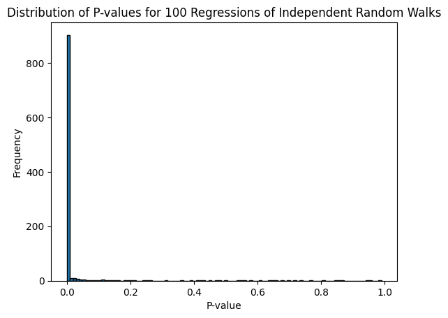
As you can see, despite having two unrelated random walks, we get a significant relationship most of the time.
To summarize, cointegration could be a great tool, allowing us to compute the hedge ratio. However, one must ensure the hypothesis of cointegration is met, meaning hypothesis testing on the stationarity of the residuals is required in order to use it. That’s where cointegration’s best friend comes into play: the stationarity test.
Several stationarity tests exist. They can be used in tandem or on their own. The two main ones are the KPSS and the ADF tests. They allow us to test if a series is likely to be stationary or not. I would advise again to read Time series Analysis if you are looking to go into the maths.
If say you suceed to find two stock which cointegrated prices, you are then able to construct a stationanry portfolio longing one share of stock A and shorting \rhau share of stock B. You can then can exploid the mean reversion properties of a stationnary process. Meaning, you will short this portfolio when it is bellow its long term mean and short it when its above its long term mean (you actually can greatly improve from this but again, we keep it simple for now).
When people use these two tools, the process is typically as follows:
- Compute the linear regression
- Perform a stationarity test on the residuals
- If the residuals are stationary, use the linear regression coefficients to get the hedge ratio
- Obtain your market-neutral portfolio
- Create entry and exit thresholds to trade on low/mid-frequency
This approach is explained by Gatev et al. in Pairs Trading: Performance of a Relative Value Arbitrage Rule. Trading the spreads is not something I will explain here but known it can be approach with stochastic calculus (OU model, …).
The pratical challenges
So far, we have a well-documented approach, complete with specified mathematics and models, that should enable us to consistently make money. So, what’s the catch? To generate consistent profits, you need to identify several pairs and trade them. I believe the identification phase is one of the most challenging aspects. If one opts for a brute force approach and applies the Augmented Dickey-Fuller (ADF) test to all possible pairs, the number of false positives will likely skyrocket.
The hedge against other players is created in this phase. The question then becomes: How will you define your universe? There are many existing stock universes that involve methods such as clustering, setting thresholds on the Hurst exponents of the spreads, and multiple stationarity tests, among others.
Additionally, there is a second challenge: you should aim to trade pairs with the fastest mean reversion speed. This is also be difficult to achieve and I will leave it an open question for now.
Conclusion
In conclusion, while the theory behind pair trading and market-neutral strategies appears robust, implementing these strategies effectively requires navigating a complex landscape of challenges. Identifying viable pairs, maintaining a truly market-neutral position, and capitalizing on mean reversion speed are just the tip of the iceberg. Each phase, from defining your universe to executing trades, demands rigorous analysis and a critical approach to data. The true test lies not only in the selection and application of models but also in our ability to adapt and refine these strategies in response to evolving market conditions. As we move forward, the subsequent posts will explore more advanced tools and techniques, aiming to enhance our understanding and execution of these sophisticated trading strategies. Stay tuned for a deeper dive into the nuances that can make or break the success of pair trading.