A closed-form filter for binary time series

Courvoisier Balthazar · July 9, 2023

Academic Project

This project is a common work with Raphael Thabut and Eric Vong. It’s a pratical implementation of A closed-form filter for binary time series by Fanaso and al.

Article presentation

Denoising data is always relevant to perform, as in reality, a lot of observations can be noised due to external effects. Most filtering methods to predict and smooth distributions relies on the assumption of the Gaussian nature of the state-space models. This is because we have closed form filters available. Even for a binary state-space model, we require Monte-Carlo strategies for prediction.

This article claims that they have found a closed form filter for the dynamic probit models with a gaussian state variable. To do so, they showed that they belong to a class of distribution, the Skew Unified Normal (SUN), whose parameters can be updated with closed expression.

They then show how the algorithm performs in practice, and how using, the properties of the SUN distribution, allows for online inference for high dimensions.

Zoom on the financial application

The articles gave an application example, using financial time series. Indeed, it focus on the analysis of two times series, the Nikkei 225 (Japanase Stock Index) and the CAC 40 (French Stock Index).

As the latter opens after the former, one can try to use the cointegration effect between the two time series to obtain relevant predictions. Our data will be composed of :

• $x_t$ where $x_t = 1$ if the Nikkei 225 opening has increased between the close value and opening value and $x_t = 0$ otherwise
• $y_t$ where $y_t = 1$ if the CAC 40 opening has increased between the close value and opening value and $y_t = 0$ otherwise

One important objective for a financial application would be to evaluate $Pr(y_t = 1 \mid x_t)$.

This can be done using a probit model. We try to infer a binary value given two parameters, the trend of the CAC 40 when the Nikkei 225 opening is negative and the shift in the trend if the Nikkei 225 opening is positive. Mathematically, this means :

$$P(y_t = 1 \mid x_t) = \Phi[F_t \theta, 1]$$

with the following notations :

• $F_t = (1, x_t)$
• $\theta = (\theta_1, \theta_2)$, $\theta_1$ being the trend and $\theta_2$ the shift

In the case of such an application, the purpose of the methods we describe in this report is to estimate the $\theta$ parameter effectively.

The SUN distribution

Gaussian models are omnipresent in mathematical models. They have very strong properties and make models simpler. Although, one important drawback is that real life distribution tends to have some sort of asymetry.

A first extension of the gaussian models, Skew Normals, has been proposed by Arellano-Valle and Azzalini (1996). Due to the fertility of this formulation, a unifying representation, the Skewed Unifyed Normals, has been proposed by them since 2006.

Given $\theta \in R^q$, we say that $\theta$ has a unified skew-normal distribution, noted $\theta \sim {SUN}_{q, h}{(\xi, \Omega, \Delta, \gamma, \Gamma)}$, if its density function $\rho{(\theta)}$ is of form:

$$\phi_q{(\theta - \xi ; \Omega)} \frac{\Phi_{h}{(\gamma + \Delta^T \overline{\Omega}^{-1} \omega^{-1} ({\theta - \xi}); \Gamma - \Delta^T \overline{\Omega}^{-1} \Delta})}{\Phi_h{(\gamma ; \Gamma)}}$$

With:

• $\phi_q{(\theta ; \Omega)}$ where $\phi_h$ is the centered gaussian density with covariance $\Omega$ matrix
• $\Phi_{h}{(\gamma ; \Gamma)}$ where $\Phi_h$ is the centered gaussian cumulative distribution function with covariance $\Gamma$
• $\Omega = \omega \overline{\Omega} \omega$ and $\overline{\Omega}$ is the correlation matrix
• $\xi$ controls the location
• $\omega$ controls the scale
• $\Delta$ defines the dependance between the covariance matrixes $\Gamma, \overline{\Omega}$
• $\gamma$ controls the truncature

The term:

$$\frac{\Phi_{h}(\gamma + \Delta^T \overline{\Omega}^{-1} \omega^{-1} (\theta - \xi) ; \Gamma - \Delta^T \overline{\Omega}^{-1} \Delta)}{\Phi_{h}(\gamma ; \Gamma)}$$

induces the skewness as it is rescaled by the term $\Phi_{h}(\gamma ; \Gamma)$

We have also the following distribution equality $\theta \overset{(d)} = \xi + \omega (U_0 + \Delta \Gamma^{-1} U_1)$ with $U_0$ independant of $U_1$ and $U_0 \sim N_q{(0, \overline{\Omega} - \Delta \Gamma^{-1} \Delta^T)}, U_1 \sim TN_h{(0, \Gamma, -\gamma)}$ truncated normal law below $-\gamma$. This representation allows for efficient computing, but we can also apply it to a probit model.

Given $y_t = (y_{1t}, \ldots, y_{mt})^T \in {(0, 1)}^m$ a binary vector and $\theta_t = (\theta_{1t}, \ldots, \theta_{pt})^T \in R^p$ the vectors of parameters. The dynamic probit model is then defined as: `

$p{(y_t \mid \theta_t)} = \Phi_m{(B_t F_t \theta_t ; B_t V_t B_t)}$ $\theta_t = G_t \theta_{t-1} + \varepsilon_t, \varepsilon_t \sim N_p{(0, W_t)}$

With $\theta_0 \sim N_{p}{(a_0, P_0)}$ with $B_t = \mathrm{diag}{(2y_{1t} - 1, \ldots, 2y_{mt} - 1)}$

This representation is equivalent to another formulation (Albert and Chib 1993) as followed:

$p{(z_t \vert \theta_t)} = \phi_m{(z_t - F_t \theta_t; V_t)}$ $\theta_t = G_t \theta_{t-1} + \varepsilon_t, \varepsilon_t \sim N_{p}(0, W_t)$

With $y_{it} = 1{z{it} > 0}$

Then, under such a dynamic, the first step filtering distribution is:

$$(\theta_1 \mid y_1) \sim SUN_{p,m}{(\xi_{1 \mid 1}, \Omega_{1 \mid 1}, \Delta_{1 \mid 1}, \gamma_{1 \mid 1}, \Gamma_{1 \mid 1})}$$

With the following parameters:

• $\xi_{1 \mid 1} = G_1 a_0$
• $\Omega_{1 \mid 1} = G_1 P_0 G_1^T + W_1$
• $\Delta_{1 \mid 1} = \overline{\Omega_{1 \mid 1}} \omega_{1 \mid 1} F_1^T B_1 s_1^{-1}$
• $\gamma_{1 \mid 1} = s_1^{-1} B_1 F_1 \xi_{1 \mid 1}$
• $\Gamma_{1 \mid 1} = s_1^{-1} B_1 \times {F_1 \Omega_{1 \mid 1} F_1^T + V_1}B_1 s_1^{-1}$
• $s_1 = (\mathrm{diag}{(F_1 \Omega_{1 \mid 1}F_1^T + V_1)})^{1/2}$

More generally, if $(\theta_t \mid y_{1:t-1}) \sim SUN_{p,m(t-1)}(\xi_{t-1 \mid t-1}, \Omega_{t-1 \mid t-1}, \Delta_{t-1 \mid t-1}, \gamma_{t-1 \mid t-1}, \Gamma_{t-1 \mid t-1})$ is the filtering distribution at $t-1$, then the predictive distribution at $t$ is $(\theta_t \mid y_{1:t-1}) \sim SUN_{p,m(t-1)}(\xi_{t \mid t-1}, \Omega_{t \mid t-1}, \Delta_{t \mid t-1}, \gamma_{t \mid t-1}, \Gamma_{t \mid t-1})$ with the following parameters:

• $\xi_{t \mid t-1} = G_t \xi_{t-1 \mid t-1}$
• $\Omega_{t \mid t-1} = G_t \Omega_{t-1 \mid t-1}G_t^T + W_t$
• $\Delta_{t \mid t-1} = w_{t-1 \mid t-1}^{-1} G_t w_{t -1 \mid t-1} \Delta_{t-1 \mid t-1}$
• $\gamma_{t \mid t-1} = \gamma_{t-1 \mid t-1}$
• $\Gamma_{t \mid t-1} = \gamma_{t-1 \mid t-1}$

And at time $t$, the filtering distribution are defined as:

• $\xi_{t \mid t} = \xi_{t \mid t-1}$
• $\Omega_{t \mid t} = \Omega_{t \mid t-1}$
• $\Delta_{t \mid t} = [\Delta_{t \mid t-1}, \overline{\Omega_{t \mid t}} \omega_{t \mid t} F_t^T B_t s_t^{-1}]$
• $\gamma_{t \mid t} = [\gamma_{t \mid t-1}^T, \xi_{t \mid t}^T F_t^T B_t s_t^{-T}]$
• $\Gamma_{t \mid t} = [[A, B], [B, C]]$
• $A = \Gamma_{t \mid t-1}$
• $B = s_t^{-1} B_t F_t \omega_{t \mid t} \Delta_{t \mid t-1}$
• $C = s_t^{-1} B_t(F_t \Omega_{t \mid t} F_t^T + V_t) B_t s_t^{-1}$
• $s_t = (\mathrm{diag}{F_t \Omega_{t \mid t} F_t^T + V_t})^{1/2}$

For the smoothing, it is available with similar forms of equations.

Particles algorithms

Particle filters are a mathematical tool used to estimate the state of a system that is described by a set of uncertain variables. It is a type of recursive Bayesian filter that estimates the state of a system by sampling a large number of “particles,” each of which represents a possible state of the system. The particles are weighted according to their likelihood of being the true state of the system, and the weighted average of the particles is used as an estimate of the state. In this section we describe two particles algorithms we used to estimate the parameters of the targeted SUN distribution : the bootstrap filter, and an optimal filter proposed by the researchers.

To obtain similar results, detailed in the fourth part of the report, we started with the same parameters and used the previously seen properties.

• $a_0 = [0, 0]$
• $P_0 = 3I_2$
• $V_t = 1$

Bootstrap filter

In a bootstrap filter, the state estimates are generated using a bootstrapping process, which involves sampling from the previous estimate of the state distribution with replacement. This means that each sample is drawn from the previous estimate, and the same sample may be drawn multiple times. The new estimate of the state is then obtained by weighting the samples according to their likelihood of being the true state.

In the specific case of our study, using the properties and the assumptions of the model, we implemented the bootstrap filter by following this pseudo code :

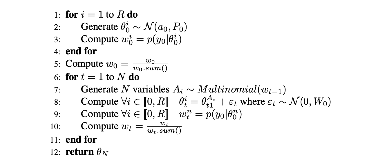
Where $W_0$ is taken as $W_0 = 0.01 I_2$ (suggested by a graphical search of the maximum for the marginal likelihood computed under different combinations via the analytical formula)

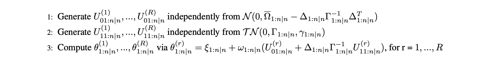
Independent and identically distributed sampling

A first filter is proposed by the researchers in the article. It uses the main properties of the SUN distribution in order to get independent and identically distributed sampling. This algorithm can be described by the following pseudo code :

Optimal filter

The optimal filter introduced by the researchers can be described by the following pseudo code, using the equations of the SUN distribution and filtering, we perform the steps :

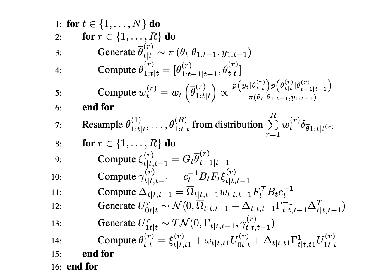
Where $G_t = \Gamma = \overline{\Omega} = I_2$ and $\omega = 0.1$, this filter leverages the SUN distribution properties detailed above. With the starting values, we have:

$$\Gamma = I_2$$

Results and Conclusion

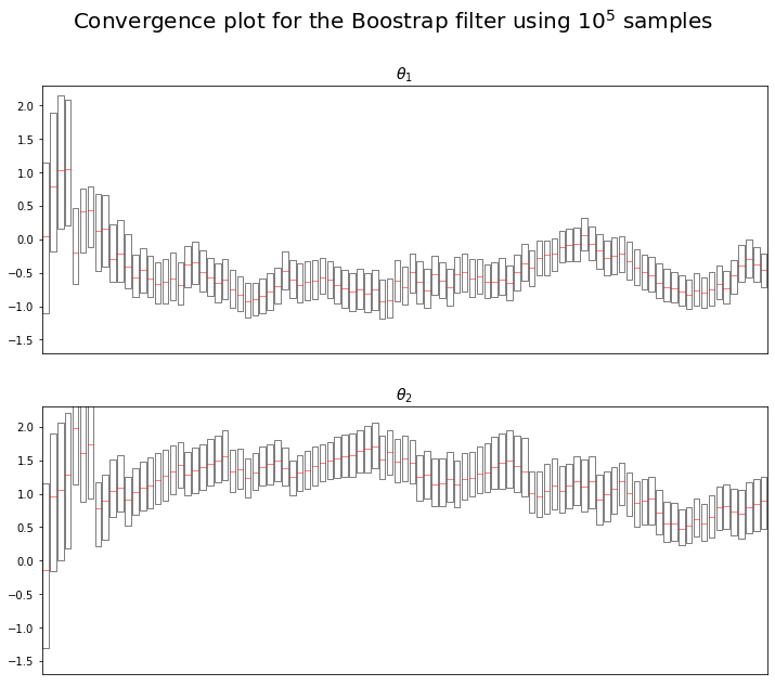
We decided to focus on the convergence of the algorithms. Plotting the convergence of the models parameter $\theta_1$ and $\theta_2$.

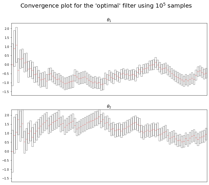
We observe similar results as the one in the paper :

• $\theta_1$ seems to tend towards -0.5
• $\theta_2$ seems to tend towards 1

One may find the same plot but for the boostrap algorithm in the Appendix. We can see the same convergence results : $\theta_1$ seems to tend towards -0.5, $\theta_2$ seems to tend towards 1.

In order to compare the accuracy of the algorithms, Fasano et al used the following procedure :

1. Compute the corresponding SUN density on a 2000*2000 sized grid of equally spaced values of $\theta_{1t}$ and $\theta_{2t}$ for each $t$ in $1,2,…,97$
2. Compute the marginal distributions of $\theta_{1t}$ (resp. $\theta_{2t}$) by summing over the values of $\theta_{2t}$ (resp. $\theta_{1t}$) and multiplying by the grid step size (this corresponds to approaching the integral of the joint density on one of the two variables by a rectangle method)
3. Run each algorithm 100 with respectively $10^3, 10^4,$ and $10^5$ particles
4. Compute the Wasserstein distance between the empirical distribution given by each algorithm and the discretized exact density
5. for each algorithm, take the median of the 100 Wasserstein distance computed

We also used this method, however due to the extensive computing time the methods required. We restrained ourselves to grids of size $100 \times 100$ and only went up to $t=50$. We ended up with the following table :

Algorithm	$\theta_1 \quad (R=10^3)$	$\theta_1 \quad (R=10^4)$	$\theta_1 \quad (R=10^5)$	$\theta_2 \quad (R=10^3)$	$\theta_2 \quad (R=10^4)$	$\theta_2 \quad (R=10^5)$
Boostrap	0.086	0.036	0.025	0.124	0.069	0.062
Optimal	0.082	0.034	0.024	0.117	0.067	0.061

We can see that our results are similar to the article’s results, and the conclusions drawn out are the same : although mild, we benefit from a better accuracy with the proposed “optimal” filter than the one we observe when using the classic bootstrap filter.
“ We also reproduced a bar plot which shows the frequency at which each algorithm dominates the other accross time.

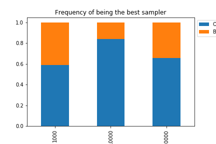
We can see the “optimal” filter has ranks above the bootstrap filter most of the time: it overperforms the bootstrap filter at frequency 0.59 for $R=10^3$, 0.84 for $R=10^4$, and 0.66 for $R=10^5$.

We also compared the performance of the algorithms throughout the time window by averaging the wasserstein distance over each of the 100 experiments for each algorithm at each time $t$, the graph below shows the results:

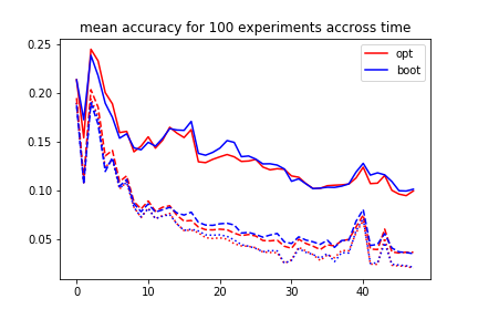
We can see that the accuracy of both algorithms decreases with time (let it be noted that here a good accuracy is a low accuracy, although this can sound confusing). Of course, we also notice throughout the study that more particles implies better results.

Finally, and because we are using Monte Carlo methods, we decided to take a look at the variance of our algrithms. We expected a smaller variance for the “optimal” algorithm. To look at the variance of the results, we simulated 100 runs with each algorithm and $10^3$ samples. We then assessed the median variance. We obtained the following results :

Algorithm	Variance of $\theta_1$	Variance of $\theta_2$
Boostrap	0.00525312	0.00937037
Optimal	0.00380095	0.00727529

As expected we have lower variance with the optimal algorithm than the boostrap algorithm. Moreover, we have a relatively small variance : $10^{-3}$ for all coefficients.

Appendix

Share: Twitter, Facebook