
Introduction
In our previous post, we explored how to fetch and store Binance candlestick data using HDF5, laying the groundwork for efficient data management in cryptocurrency research. Efficient data handling is crucial when dealing with large datasets, especially in the fast-paced world of crypto trading.
Now, we’re taking the next step in our journey by delving into the analysis of this data. This is the first part of a three-part series where we’ll dive deep into estimating Bitcoin’s volatility using different methods.
Terminology Alert : Volatility measures how much and how quickly the value of an asset changes.
It’s important to note that volatility is not directly observable. It’s a hidden variable that must be estimated from market data. Its value can vary depending on the estimation model used, making it a crucial yet complex component in financial analysis.
There are two main types of volatility:
-
Realized Volatility: Calculated from past market prices, it reflects the asset’s actual price movements over a specified period.
-
Implied Volatility: Derived from the market price of a traded derivative, especially options. It represents the market’s expectation of future volatility.
Why this difference ? Well, it happens volatility is far easier to predict than returns themselves. For options or other financial products, the future value of the volatility (meaning the future behaviour of the asset) is more usefull. Thus, the market will use the volatility expectancy for those products. In this post, we will focus on the realized volatility.
Why Analyze Bitcoin’s Realized Volatility ?
Understanding realized volatility is crucial, especially when dealing with highly volatile assets like Bitcoin. Realized volatility measures the degree of variation in an asset’s past price movements over a specific period. Studying it provides valuable insights into the asset’s risk profile and helps in making informed decisions. Here’s why analyzing realized volatility is essential:
- Risk Assessment and Management: Realized volatility is a key indicator of the risk associated with an asset. By analyzing how much Bitcoin’s price has fluctuated in the past, traders and investors can gauge the potential risk of future price movements.
- Strategic Trading Decisions: Studying realized volatility can help traders develop effective trading strategies by recognizing periods of high or low volatility to choose appropriate trading approaches (e.g., trend following in high volatility, mean reversion in low volatility).
- Option Pricing and Derivative Valuation: Since volatility is a hidden variable and not directly observable, realized volatility serves as an essential estimate.
- Getting Risk-Adjusted Returns: Evaluating whether the potential returns justify the risks based on realized volatility.
In essence, studying realized volatility is not just an academic exercise—it’s a practical necessity. It equips traders and investors with the knowledge to navigate the complexities of the financial markets, particularly the dynamic and often unpredictable cryptocurrency landscape. By acknowledging that volatility is a hidden variable dependent on estimation models, we can appreciate the importance of selecting appropriate methods to measure and interpret it. This understanding ultimately leads to better risk management, more effective trading strategies, and informed decision-making in the pursuit of financial goals.
Preparing Binance Bitcoin Data for EWMA in Python
Before we can estimate volatility, we need to prepare our data. The database we will use is the one we created in this post.
Loading Data from HDF5
First, let’s load the Bitcoin data we previously stored in our HDF5 file.
import pandas as pd
import numpy as np
import matplotlib.pyplot as plt

# Load the data from the HDF5 file
df = pd.read_hdf('data/crypto_database.h5', key='BTCUSDT')
This will give us access to the Bitcoin candlestick data with 1-minute granularity.
Data Cleaning and Preprocessing
Ensuring data quality is paramount. We’ll check for missing values and ensure that the data types are appropriate.
# Check for missing values
print(df.isnull().sum())

# Convert 'Open_Time' to datetime if not already done
df.reset_index(inplace=True)
df['Open_Time'] = pd.to_datetime(df['Open_Time'])

# Set 'Open_Time' as the index
df.set_index('Open_Time', inplace=True)
Taking a look at the data
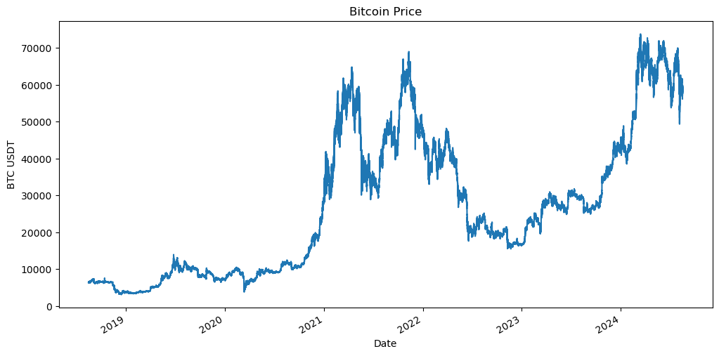
Let’s ensure we have good quality data by plotting the evolution of the Bitcoin Price.
# Plot the log returns
plt.figure(figsize=(12, 6))
df['Close'].plot()
plt.title('Bitcoin Price')
plt.xlabel('Date')
plt.ylabel('BTC USDT')
plt.show()
Calculating Bitcoin Log Returns in Python
Logarithmic returns, or log returns, can be preferred over simple returns for several reasons:
- Time Additivity: Log returns are additive over time, which simplifies calculations.
- Normality: They often better approximate a normal distribution, which is a common assumption in financial models.
- Symmetry: Log returns treat upward and downward movements symmetrically.
The formula for log returns is:
\[r_t = \ln\left(\frac{P_t}{P_{t-1}}\right)\]Where:
- $ r_t $ is the log return at time $ t $.
- $ P_t $ is the price at time $ t $.
Let’s calculate the log returns using the ‘Close’ price. While this approach is common, it’s important to note that volatility estimation doesn’t have to rely solely on the ‘Close’ price; other data points like the ‘Open’, ‘High’, and ‘Low’ during a time interval are also meaningful and can provide additional insights. However, for simplicity in this post, we’ll only use the ‘Close’ price.
# Calculate log returns
df['log_returns'] = np.log(df['Close'] / df['Close'].shift(1))

# Drop the NaN value created by the shift
df.dropna(subset=['log_returns'], inplace=True)
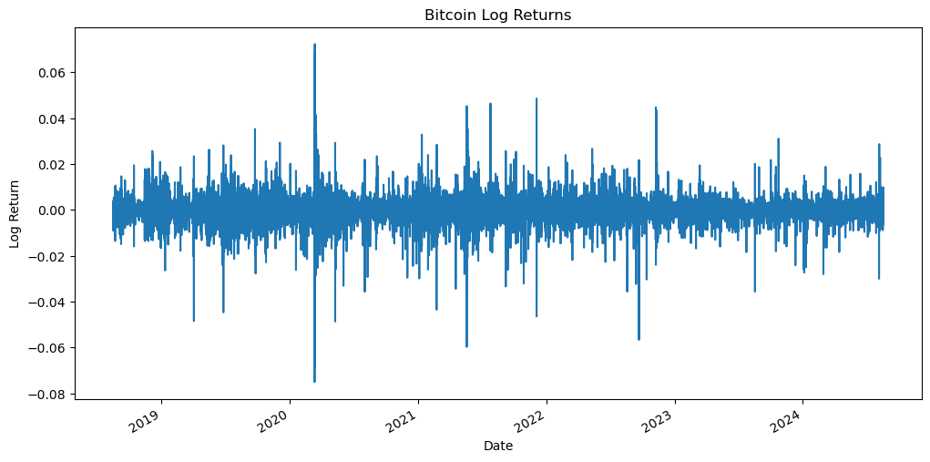
Now, let’s visualize the log returns to get a sense of their behavior.
# Plot the log returns
plt.figure(figsize=(12, 6))
df['log_returns'].plot()
plt.title('Bitcoin Log Returns')
plt.xlabel('Date')
plt.ylabel('Log Return')
plt.show()
Estimating Bitcoin Volatility with EWMA
Introducing the EWMA Method
The Exponentially Weighted Moving Average (EWMA) is a powerful statistical technique that assigns exponentially decreasing weights to past observations, giving more significance to recent data points. This responsiveness to the latest market information makes EWMA particularly valuable in volatile markets like cryptocurrency, where conditions can change rapidly.
EWMA was popularized by J.P. Morgan in the early 1990s through their development of the RiskMetrics system. RiskMetrics provided a standardized framework for measuring and managing market risk, introducing EWMA as an effective method for estimating volatility. John Hull’s book “Options, Futures, and Other Derivatives” discusses EWMA as an effective method for volatility estimation. By emphasizing recent price movements without entirely discarding older data, EWMA captures the persistence and clustering of volatility often observed in financial time series.
The EWMA volatility is calculated using the formula:
\[\sigma_t^2 = \lambda \sigma_{t-1}^2 + (1 - \lambda) r_t^2\]Where:
- $ \sigma_t^2 $ is the variance at time $ t $.
- $ \lambda $ is the decay factor (0 < $ \lambda $ < 1).
- $ r_t $ is the return at time $ t $.
Setting the Decay Factor (Lambda)
The choice of the decay factor $ \lambda $ determines how quickly the weights decrease. A commonly used value is $ \lambda = 0.94 $, as suggested by RiskMetrics. A higher $ \lambda $ gives more weight to older observations, while a lower $ \lambda $ emphasizes recent returns more heavily.
Step-by-Step Calculation
Using pandas, we can implement the EWMA volatility estimation easily.
# Set the decay factor
lambda_ = 0.94
alpha = 1 - lambda_

# Calculate the EWMA variance
df['ewma_variance'] = df['log_returns'].ewm(alpha=alpha, adjust=False).var()

# Calculate the EWMA volatility
df['ewma_volatility'] = np.sqrt(df['ewma_variance'])
Visualization
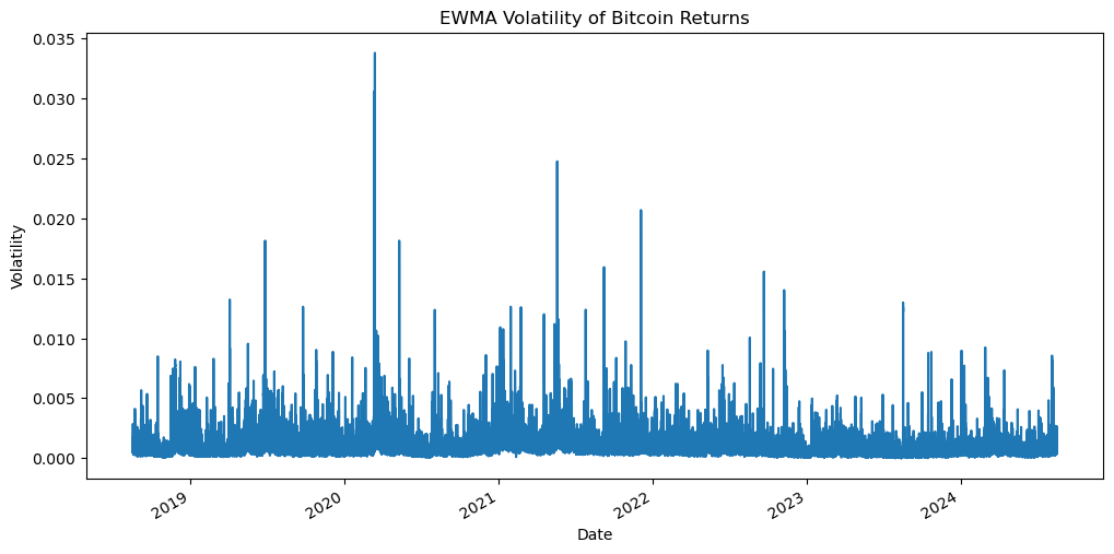
Let’s plot the EWMA volatility to visualize how it changes over time.
# Plot the EWMA volatility
plt.figure(figsize=(12, 6))
df['ewma_volatility'].plot()
plt.title('EWMA Volatility of Bitcoin Returns')
plt.xlabel('Date')
plt.ylabel('Volatility')
plt.show()
Analyzing the Results
By analyzing the plot, we can identify periods of sharp volatility spikes, which signal higher risk and potentially greater reward opportunities. These spikes are often triggered by significant market events or news impacting Bitcoin. This behavior is known as volatility clustering, where high-volatility periods are followed by similarly turbulent periods, while low-volatility phases exhibit smaller, more stable fluctuations.
EWMA Volatility: Advantages and Limitations
- Responsiveness: EWMA adjusts quickly to changes, making it suitable for volatile markets.
- Simplicity: It’s straightforward to implement and doesn’t require complex modeling.
- Weighted Data: By giving more importance to recent data, EWMA provides a more current view of market volatility.
- Easy Online Learning: EWMA is well-suited for real-time or online learning, where data is processed sequentially. In production environments, where data arrives continuously, this feature ensures the system can easily adapt without reprocessing the entire dataset each time.
These characteristics make EWMA a highly practical tool for production applications, especially in environments where real-time data processing is critical. Yet it has some important limitations that should be considered, especially when thinking about future predictions:
-
No Predictive Power for Future Volatility: The EWMA estimator is not suitable for predicting future volatility. When simulating future values of the model, the expectation $ E[\sigma_{t+h}] $ tends to 0 as $ h $ increases, meaning the model effectively predicts no future volatility (assuming $ E[ r_t] = 0 $ ). This limitation arises because EWMA only reacts to past data without incorporating any forward-looking information or structural changes in the market.
-
Constant Decay Factor: The choice of the decay factor $ \lambda $ is critical to the model’s performance. However, EWMA uses a constant $ \lambda $, which assumes that the rate at which past data becomes less relevant is fixed over time. This might not be realistic during periods of sudden market regime shifts, where volatility patterns change dramatically.
-
Sensitivity to Large Shocks: While EWMA adapts to volatility changes, it might still overreact to short-term shocks. Large price movements (like flash crashes) can disproportionately affect the estimated volatility in the short term, without accounting for whether these movements represent structural shifts or noise.
Lastly, as explained by Collin Bennet in his book Trading Volatility Exponentially weighted volatility models struggle to account for recurring volatility-inducing events like earnings reports. Just before an earnings announcement—when future volatility is expected to rise—the model places the least weight on previous earnings-related volatility spikes. Conversely, right after the earnings event—when future volatility is likely to decrease—the model assigns the most weight to these prior events. However, these models may still have some applicability when analyzing indices.
Due to these limitations, the EWMA method is suitable only for historical analysis and not for forecasting future volatility. More advanced models, like GARCH, are better suited for predicting future volatility because they account for the persistence and reversion tendencies in volatility over time.
Conclusion and Next Steps
In this post, we’ve introduced the concept of volatility and its importance in financial markets, particularly for Bitcoin. We’ve shown how to estimate volatility using the EWMA method, which provides a responsive and practical approach for traders and analysts.
This is just the beginning. In the next posts of this series, we’ll explore more sophisticated methods like GARCH models for volatility estimation.
Stay tuned for deeper insights into the fascinating world of financial volatility analysis!
Additional Resources
- Code Repository: GitHub Link
- Adviced Reading: John Hull’s Options, Futures, and Other Derivatives and Collin Bennet’s Trading Volatility
Feel free to share your thoughts or ask questions in the comments below. I encourage you to experiment with the code, try different decay factors, and see how it affects the volatility estimates.
I’d love to hear your thoughts! Share your feedback, questions, or suggestions for future topics in the comments below.
Happy analyzing, and as always, may your trading strategies be well-informed!